Standalone version
Command-line tool
Roadmap
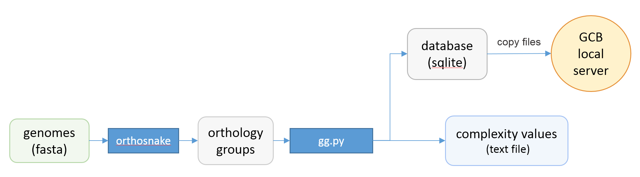
Standalone version should be used when the user wants to work with a custom set of genomes. Command-line scripts are provided to: calculate complexity profile, generate subgraphs, generate a database which can be imported to browser-based GUI application. Scheme of actions and scripts is shown below.
Prerequisites
Conda
Please refer to the installation guide. Select Python3 version.
Snakemake
Installation instrctions are here.
Python 3.6 or later
Comes with conda.
Graphviz and pygraphviz libraries
Can be installed via conda:
conda install -c anaconda graphviz
conda install -c conda-forge pygraphviz==1.7
gene_graph_lib Python3 module
Can be installed by running:
pip3 install gene_graph_lib
Orthogroup inference
Orthogroup inference is the first step in the standalone analysis. We recomend using our orthosnake pipeline for inference of orthogroups, because GCB requires some special formating of the files.
Orthosnake pipeline
INPUT: Fasta-formated files with .fna extension, one file per genome
OUTPUT: orthogroups file `Orthogroups.txt` in OrthoFinder format
Steps:
- Clone or download orthosnake GIT repository: https://github.com/paraslonic/orthosnake
- Put fasta-formated genome files in
fnafolder of the orthosnake folder.- Rut snakemake with
--use-condaand other appropriate options
The following code will run analysis of the test dataset (three plasmids):
git clone https://github.com/paraslonic/orthosnake.git
cd orthosnake
cp test_fna/* fna # copy test fasta files with three plasmids
snakemake -j 4 --use-conda
Here, we used snakemake with parameters specifying the number of available cores (-j 4), and using conda environments (--use-conda). During the first start of the pipeline, it will take about ten minutes to install the necessary programs into the conda environments.
If genome files have extension, other than .fna (e.g., *.fasta) , please rename them. For example, to change the file extension from .fasta to .fna, run:
for i in fna/*.fasta; do mv $i fna/$(basename $i .fasta).fna; done
Orthosnake pipeline performs the following steps:
Fasta headers are modified, to satisfy the requirement of the Prokka
- symbols other than alphanumericals and ‘_’ are converted to ‘_’
- if header is longer than 20 symbols, it is cropped to the first 18 symbols, and dots are added to the end (e.g.,
gi|15829254|ref|NC_002695.1becomesgi|15829254|ref|NC..)Annotation with Prokka.
Genebank files converted to amino acid fasta files.
Orthogroups are inferred with OrthoFinder.
When amino acid fasta files are generated from genebank files, information regarding location and product is included in headers in the following format: genome_name|numerical_id|start|end|product. Please note this if you want to perform orthogroups inference without using orthosnake.
Building a graph and complexity estimation
INPUT: orthogroups file `Orthogroups.txt` in OrthoFinder format
OUTPUT: graph-based representation of genomes (sqlite database), complexity values (text file)
To perform the basic analysis, you should install geneGraph:
git clone https://github.com/DNKonanov/geneGraph
cd geneGraph
and run:
python3 gg.py -i [orthogroups file] -o [output] --reference [name of the reference genome]
Parameters:
-i– path to orthogroups file in OrthoFinder format.
-o– path and name prefix for output files
--reference– name of the reference genome (its filename without extension), used for complexity estimation. This parameter can be skipped, in this case, the complexity values for all genomes in the set will be estimated (this can take a lot of time).
Optional parameters:
--window– size of the window used in the complexity estimation (default is 20). Only the paths inside the window increase the value of complexity.
--genomes_list– a text file containing the names of the genomes that will be used to calculate the complexity. Useful for analysis of parts of genomes, such as phylogenetic tree clades, for their subsequent comparison.
--coalign– a binary value (True/False) that determines whether to perform the step of selecting the optimal genomes orientation. It can take a lot of time when using a large number of draft genomes (5 hours for 1000 draft genomes).
Advanced complexity estimation algorithm settings (practically not used):
--iterations– number of iterations in algorithm (default is 500)
--min_depth– minimum length of deviating path (default is 0)
--max_depth– maximum length of deviating path (default is inf)
What this command does:
- parses OrthoGroups.txt
- creates graph file in sif-format and additional information about genes, their contextes, etc.
- creates SQLite database used in GCB
- computes complexity profiles for ALL genomes in the dataset and fills the DB
- dumps graph object for fast access
- all operations are executed by two ways: with deletion of paralogues, and with artificial orthologization
Main output files are:
<output>.db- SQLite database containing graph and complexity values, paralogues genes are skipped.<output>_pars.db- SQLite database conatining graph and complexity values, paralogues genes are orthologized.[reference genome]/prob_window_complexity_contig_[contig].txt- text file containing complexity values for each contig in the reference genome.<output>_context.sif- number of unique contexts, computed for each node in graph<output>_genes.sif- list of all genes (nodes) from all genomes, with coordinates and Prokka annotations
Where, <output> is what was specifiend in -o option, while running gg.py.
Local GCB server
Installation
First, clone or download git repository:
git clone https://github.com/DNKonanov/GCB.git
Then, install dependencies:
pip3 install -r requirements.txt

conda install -c conda-forge graphviz pygraphviz==1.7

git clone https://github.com/paraslonic/orthosnake

git clone https://github.com/DNKonanov/geneGraph
Usage
Add data
To generate a dataset for GCB you need to run GeneGraph, a command-line tool to generate graphs and complexity profiles.
Suppose, we have a number of *.fna files for 100 different genomes of Mycoplasma.
First, orthogroup file OrthoGroups.txt should be generated with orthosnake. OrthoGroups.txt will be in orthosnake/Results folder.
Next, use gg.py script from geneGraph to generate GCB databases:
python gg.py -i [path to OrthoGroups.txt] -o Mycoplasma
Now move the created Mycoplasma folder to GCB/data. If there is no data folder in GCB root folder, just create it with mkdir data.
Start server
To start GCB server on your computer type in GCB_package folder this:
python3 gcb_server.py
Open 127.0.0.1:8000 or localhost:8000 in your web-browser and use GCB.
Restart the sever after adding new datasets.
Complete step-by-step example
Here we will install all prerequisites and software needed for the analysis, and will add a new dataset to a local GCB server.
Following folders will be created:
orthosnake- Snakemake pipeline to infere orthogroups. We will download genomes from the RefSeq here.
geneGraph- console applications needed to build the graph-based represenatation of genomes.
mpneumoniae- a project folder, here the graph representation will be build for 5 Mycoplasma pneumoniae genomes.
GCB- local server application, this folder contains all datasets.
Note: we will work in the home directory, consider using other folders according to your preference.
Install conda
Install conda if you have not done it previously, for example by following miniconda installation guide.
Create conda environment
To create conda environment for GCB and install snakemake into this environment, run:
conda install -c conda-forge mamba
mamba create -c conda-forge -c bioconda -n gcb snakemake
conda activate gcb
Download orthosnake
Orthosnake will be needed to infere orthogroups:
cd ~
git clone https://github.com/paraslonic/orthosnake.git
cd orthosnake
Download genomes
Get file with RefSeq genomes information:
wget ftp://ftp.ncbi.nlm.nih.gov/genomes/refseq/assembly_summary_refseq.txt
Download 5 complete genomes of M. pneumoniae from the RefSeq database:
grep "Mycoplasma pneumoniae" assembly_summary_refseq.txt | grep "Complete" | awk -F "\t" '{print $20}' | awk 'BEGIN{FS=OFS="/";filesuffix="genomic.fna.gz"}{ftpdir=$0;asm=$10;file=asm"_"filesuffix;print ftpdir,file}' > complete_genomes.url
head -5 complete_genomes.url > selected_genomes.url
wget $(cat selected_genomes.url)
Move this genomes to fna folder (inside orthofinder folder):
gunzip *.gz
mv *.fna fna
Run orthofinder
Note: Installation of prokka and orthofinder will be performed during the first run.
Run orthofinder in 4 threads (will take around 20-30 minuttes):
snakemake -j 4 --use-conda
We have inferred orthogroups, they are located in Results/Orthogroups.txt file.
Download geneGraph console tools
geneGraph is needed to build a grpah-based representation of genomes:
cd ~
git clone https://github.com/DNKonanov/geneGraph.git
pip3 install gene_graph_lib
Build a graph-based representation of genomes:
cd ~
mkdir mpneumoniae
cd mpneumoniae
cp ~/orthosnake/Results/Orthogroups.txt .
python ~/geneGraph/gg.py -i Orthogroups.txt -o mycoplasma_pneumoniae
Analysis will take about a minute.
Install GCB local web server
GCB application is needed to visualize genomes in a graph-based form. All datasets are located in its data subfolder:
cd ~
git clone https://github.com/DNKonanov/GCB.git
cd GCB
pip3 install -r requirements.txt
conda install -c conda-forge graphviz pygraphviz==1.7
Copy results of geneGraph run into ``data`` folder:
mkdir data
cp -r ~/mpneumoniae/mycoplasma_pneumoniae/ data
Run local server:
python3 gcb_server.py
Open http://127.0.0.1:8000/ in a web browser, select mycoplasma_pneumoniae in Organism selecter in left panel, work with GCB.